Rules and Constraints Working Together

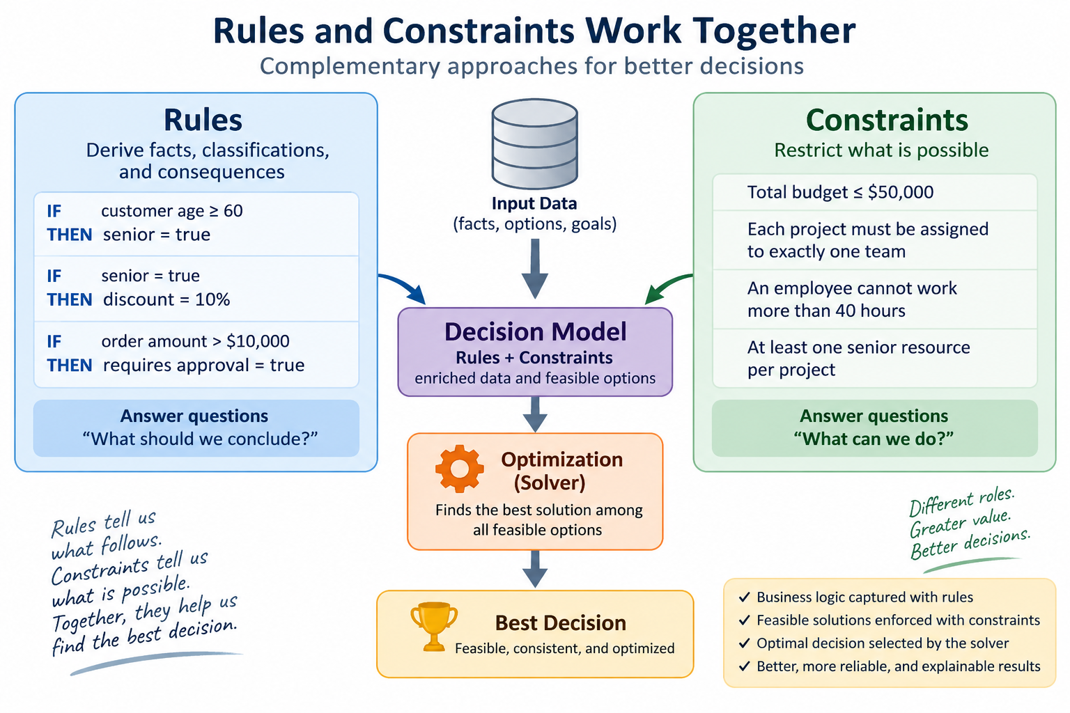
People who build decision systems with business-rules products often regard constraints as a special case of rules, especially without experience using optimization tools. I asked ChatGPT about the difference and received a useful starting point.

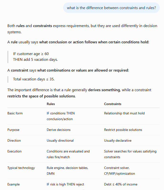
Both rules and constraints express requirements in decision systems, but they play different roles. The following sections examine those differences when designing and executing decision models.

Problem definition

When we define a decisioning problem, we first define all decision variables. If a decision variable is already known, we initialize it with an input or default value. If it is unknown - an output or intermediate variable - we specify its possible values, or domain. We then define the relationships between the decision variables using rules, constraints, or both.

Rules execution versus constraint posting

Here is the principal difference. Rules are usually executed immediately, validating the current values of the decision variables involved. Constraints are usually not executed; they are posted, or memorized, so they are checked automatically whenever one of their decision variables changes. Those variables may not yet be known and can still take any value from their domains.

After execution, rules are forgotten. Constraints remain active.

Input validation

Rule-based systems usually execute separate validation rules to confirm that input data is consistent before applying problem-resolution rules.

When constraints are posted, initial constraint propagation can automatically exclude apparently inconsistent values from the domains of the variables involved. If propagation empties the domain of even one decision variable, posting fails. Inspecting the result can therefore validate input and identify which constraints were violated and why.

The best validation results come from using rules and constraints together in one decision-making system.

Problem resolution

Pure rule-based systems

Over the last 25 years, rule-based systems have moved away from RETE engines, which many business users found too complex, and now commonly rely on sequential rule engines. This approach requires rules for every relevant combination of decision variables in order to produce a definitive outcome. It concentrates on how to reach the expected result.

Despite their user-friendliness, many such systems are therefore procedural rather than genuinely declarative. That increases the burden of building and maintaining decision models, and limits their functional capabilities.

Pure constraint-based systems

Constraint and linear or mixed-integer programming solvers have been used for more than fifty years to represent complex real-world problems in many industries. They let modelers concentrate on what a decision model should achieve, leaving problem resolution to a search method. They can find and compare multiple feasible solutions or an optimal solution, unlike the single result usually produced by a rule-based system.

However, optimization tools commonly use specialized languages such as OPL, AMPL, and MiniZinc, or APIs for Python, Java, and C++. Constraint-based decision models therefore tend to remain in the hands of technical experts.

Again, the strongest overall results come from combining rules and constraints in the same decision-making system.

Rules and constraints in the same decision model

As a practical developer of decision-making systems, I have long wanted integrated rule engines and optimization solvers. In 2011, I developed a Rule Solver that transformed a business-rule decision model into a constraint-satisfaction problem executable by a constraint solver. Although the approach attracted substantial interest, pure constraint solvers have monotonicity limitations. In practical systems, this meant splitting a decision model into separate rule-based and constraint-based parts and orchestrating them as separate decision services.

Later, OpenRules enhanced Rule Solver so off-the-shelf constraint and linear solvers could resolve rule-based decision models. Specialized decision tables supported constrained-variable creation and constraint posting, including global constraints. In practice, those tables could still be awkward for intermediate variables in complex constrained expressions, and required more optimization knowledge than many business users have.

In August 2026, OpenRules announced a redesigned Rule Solver with an expression language that integrates rules and constraints within the same decision model. A business user can define constrained, unknown variables alongside known variables in the Business Glossary, and can express ordinary and global constraints intuitively in traditional decision tables. Explore the approach in the OpenRules Rule Solver Zebra Puzzle example.

Example: Where is Zebra?

The September 2026 Zebra Puzzle challenge is a useful comparison point. Problems with nontrivial logic and many combinations of decision variables are hard to solve with business-rules-only tools. A typical approach is to generate a large number of possible test cases, then select a feasible or optimal one. For a large search space, this can lead to combinatorial explosion.

The challenge has four published solutions: IBM Bob with CPLEX, OR-Tools CP-SAT, a MILP formulation using CBC, and the latest Rule Solver.

Alex Fleischer used IBM Bob and OPL CPLEX, an AI coding agent that generated correct OPL CPLEX code. It uses the global allDifferent constraint and represents the relationship “Kools are smoked next to the house where the horse is kept” as abs(kools - horse) == 1.

Alireza Soroudi used OR-Tools CP-SAT to create Python code. It also uses predefined global allDifferent constraints and expresses part of the Kools-and-horse relationship as:

model.add(x_assign["cigarettes", "Kools"] - x_assign["pets", "Horse"] >= -1)

Adam DeJans Jr. used a MILP formulation and the textbook encoding of all-different constraints:

for each category, value:      sum over houses  x[category, value, house] == 1
for each category, house:      sum over values   x[category, value, house] == 1

For “Kools are smoked in the house next to the horse,” the model encodes adjacency for each house against its actual neighbors:

for each house h:  x[smoke, Kools, h] <= sum of x[pet, Horse, h'] for h' adjacent to h

All three approaches resolve the puzzle correctly and demonstrate useful syntactic representations of complex logical constraints. Still, people with less optimization experience - especially business users - may find API-based models less intuitive than familiar decision tables.

Rule Solver implementation

The Rule Solver model starts with the Business Glossary.

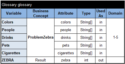
It defines ProblemZebra with five input arrays - Colors, People, Drinks, Pets, and Cigarettes - and their elements. The Domain column specifies that each array contains decision variables whose possible values are the still-unknown house numbers 1 through 5.

The corresponding test data are concise.

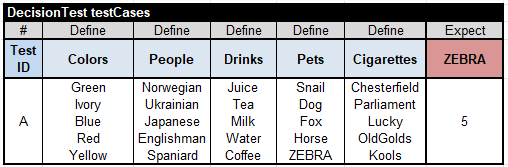
All problem constraints appear in a single decision table.

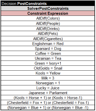
The Kools-and-horse constraint can be written directly as:

(Kools = Horse + 1) OR (Kools = Horse - 1)

These tables can be created in Excel and executed with the standard test.bat batch file. The result is immediate:

Green[5] Ivory[4] Blue[2] Red[3] Yellow[1]
Norwegian[1] Ukrainian[2] Japanese[5] Englishman[3] Spaniard[4]
Juice[4] Tea[2] Milk[3] Water[1] Coffee[5]
Snail[3] Dog[4] Fox[1] Horse[2] ZEBRA[5]
Chesterfield[2] Parliament[5] Lucky[4] OldGolds[3] Kools[1]

Thus, Zebra lives in house 5.

This integrated rules-and-constraints approach is designed to retain the simplicity and understandability of decision tables while adding optimization capabilities. Rule Solver decision models also inherit the wider Decision Intelligence Platform capabilities: a business-oriented IDE with a test harness and rule debugger, deployment options, security, and integration with existing environments.

To learn more, visit DecisionCAMP 2026 and watch “Democratizing Optimization through Decision Intelligence Platforms.”