
The July 2024 Smart Investment challenge asks how to allocate $10,000 across four stocks. Every stock must receive at least $1,000, no stock may receive more than $5,000, shares are purchased in whole units, and the objective is to maximize projected one-year gain.
This is a tiny integer linear program. The interesting part is not solver difficulty; it is translating a business statement such as “put between $1,000 and $5,000 in each stock” into the actual integer share decisions implied by market prices.
I solved the resulting model with HiGHS through SciPy’s milp interface.
Optimal allocation
| Stock | Shares | Current price | Amount invested | Projected price | Projected value | Gain |
|---|---|---|---|---|---|---|
| ABC | 120 | $25 | $3,000 | $35 | $4,200 | $1,200 |
| XYZ | 20 | $50 | $1,000 | $60 | $1,200 | $200 |
| TTT | 10 | $100 | $1,000 | $125 | $1,250 | $250 |
| LMN | 200 | $25 | $5,000 | $40 | $8,000 | $3,000 |
| Total | $10,000 | $14,650 | $4,650 |
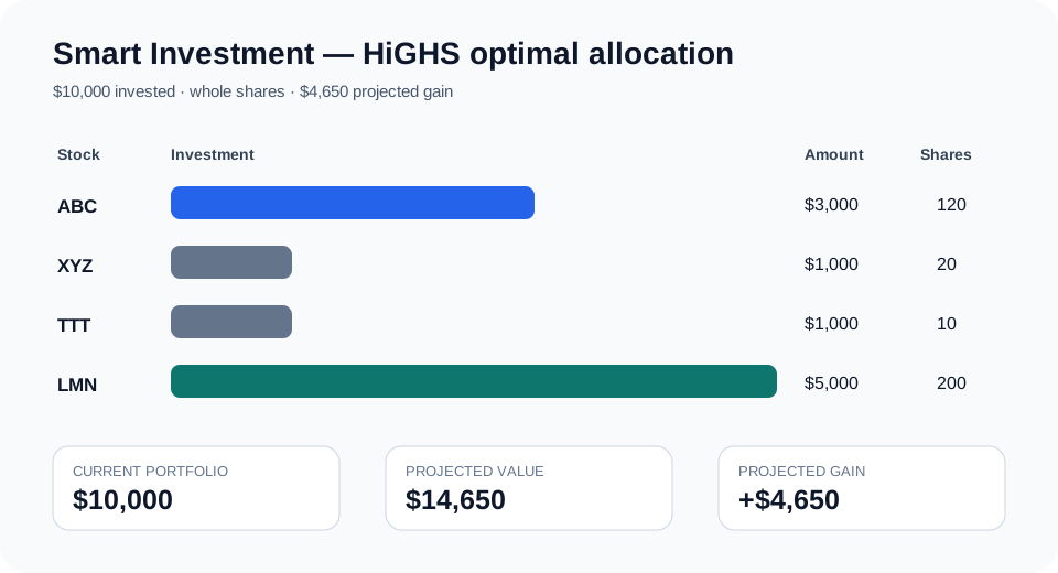
The solution allocates the required minimum to XYZ and TTT, pushes LMN to its $5,000 cap, and places the remaining $2,000 above ABC’s minimum into ABC.
This lines up with the economics of the data. The projected percentage gains are:
| Stock | Projected return on current price |
|---|---|
| LMN | 60% |
| ABC | 40% |
| TTT | 25% |
| XYZ | 20% |
Once the $1,000 minimum in each stock is satisfied, extra dollars should flow first to LMN and then ABC, subject to the $5,000 cap and whole-share restrictions. HiGHS confirms that intuition and proves the integer solution optimal.
MILP formulation
Let x_i be the number of shares purchased of stock i. Each x_i is a nonnegative integer.
For each stock, current spend is p_i x_i and projected gain is (q_i - p_i) x_i, where p_i is current price and q_i is projected price.
The objective is:
max sum_i (q_i - p_i) x_isubject to the portfolio budget:
sum_i p_i x_i <= 10000and the per-stock investment bounds:
1000 <= p_i x_i <= 5000 for every stock iwith:
x_i integer and x_i >= 0Solving it with HiGHS
import numpy as np
from scipy.optimize import milp, LinearConstraint, Bounds

price = np.array([25, 50, 100, 25], dtype=float)
projected = np.array([35, 60, 125, 40], dtype=float)
gain = projected - price

rows = [price.copy()]
lower = [-np.inf]
upper = [10000]

for i in range(4):
    row = np.zeros(4)
    row[i] = price[i]
    rows.append(row)
    lower.append(1000)
    upper.append(5000)

result = milp(
    c=-gain,
    integrality=np.ones(4),
    bounds=Bounds(np.zeros(4), np.full(4, np.inf)),
    constraints=LinearConstraint(
        np.vstack(rows), np.array(lower), np.array(upper)
    ),
)

print(result.x)
print(-result.fun)
The verified solver output is:
Shares = [120, 20, 10, 200]
Maximum projected gain = 4650
MIP gap = 0.0
Branch-and-bound nodes = 1
The current value of the portfolio is exactly $10,000 and its projected one-year value is $14,650.
A useful modeling detail
If fractional shares were allowed, this would be a linear program. Requiring whole shares makes it an integer program, but the model does not otherwise become complicated. That is a useful reminder: discrete business decisions do not automatically require complicated algorithms. Often the cleanest implementation is simply to state the economics and constraints directly and let a general-purpose solver handle the combinatorics.
The same model can be extended with sector exposure limits, transaction costs, cardinality constraints, risk budgets, tax lots, or scenario-based downside constraints.
Solution by Adam DeJans Jr. using HiGHS.
Join the discussion
Sign in with GitHub to leave a comment.