
The June 2019 Map Coloring with Violations challenge takes the classic map-coloring problem and deliberately makes perfect feasibility impossible. Six neighboring countries must use only three colors. Belgium, France, Germany, and Luxembourg form the difficult core: Belgium, France, and Germany already require the three different colors, so Luxembourg must match one of them.
The challenge assigns a cost to each of Luxembourg’s possible same-color violations:
| Potential violation | Cost |
|---|---|
| France–Luxembourg | $257 |
| Luxembourg–Belgium | $568 |
| Luxembourg–Germany | $904 |
This is a nice example of soft constraints in MILP. Hard adjacency rules remain hard; the unavoidable Luxembourg conflict is represented by binary violation variables and priced in the objective.
I solved the model with HiGHS through SciPy’s milp interface.
Optimal coloring
One optimal coloring returned by HiGHS is:
| Country | Color |
|---|---|
| Belgium | Red |
| Denmark | Red |
| France | Blue |
| Germany | Green |
| Luxembourg | Blue |
| Netherlands | Blue |
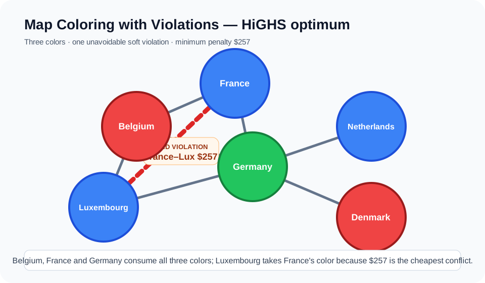
France and Luxembourg share blue, creating the $257 France–Luxembourg violation. Every hard border remains properly colored.
The total penalty is therefore:
$257HiGHS proves that this is optimal. Because Belgium, France, and Germany form a three-country triangle, they consume all three available colors. Luxembourg borders all three, so it must match one of them. The cheapest allowed conflict is the $257 France–Luxembourg edge.
MILP formulation
For each country i and color k, define:
x[i,k] = 1 if country i receives color kEvery country receives exactly one color:
sum_k x[i,k] = 1 for every country iFor a hard border (i,j), the two countries cannot share color k:
x[i,k] + x[j,k] <= 1 for every hard edge and color kFor each priced soft border e = (i,j), define a binary variable y[e,k] that activates when both endpoints use color k:
y[e,k] >= x[i,k] + x[j,k] - 1The objective minimizes the cost of all activated violations:
min sum_e cost[e] * sum_k y[e,k]Since each country receives only one color, at most one y[e,k] can be active for a given border.
Solving it with HiGHS
import numpy as np
from scipy.optimize import milp, LinearConstraint, Bounds

countries = [
    "Belgium", "Denmark", "France",
    "Germany", "Luxembourg", "Netherlands",
]
colors = ["Blue", "Red", "Green"]

# Borders that must remain different.
hard_edges = [
    ("Belgium", "France"),
    ("Belgium", "Germany"),
    ("Belgium", "Netherlands"),
    ("Denmark", "Germany"),
    ("France", "Germany"),
    ("Germany", "Netherlands"),
]

# The three unavoidable/costed Luxembourg alternatives from the challenge.
soft_edges = [
    ("France", "Luxembourg", 257),
    ("Luxembourg", "Germany", 904),
    ("Luxembourg", "Belgium", 568),
]

x = {
    (country, color): i
    for i, (country, color) in enumerate(
        (country, color)
        for country in countries
        for color in colors
    )
}

y = {}
next_var = len(x)
for e in range(len(soft_edges)):
    for color in colors:
        y[e, color] = next_var
        next_var += 1

n = next_var
objective = np.zeros(n)
for e, (_, _, penalty) in enumerate(soft_edges):
    for color in colors:
        objective[y[e, color]] = penalty

rows, lower, upper = [], [], []

# Exactly one color per country.
for country in countries:
    row = np.zeros(n)
    for color in colors:
        row[x[country, color]] = 1
    rows.append(row)
    lower.append(1)
    upper.append(1)

# Hard borders cannot match.
for a, b in hard_edges:
    for color in colors:
        row = np.zeros(n)
        row[x[a, color]] = 1
        row[x[b, color]] = 1
        rows.append(row)
        lower.append(-np.inf)
        upper.append(1)

# Soft-border activation.
for e, (a, b, _) in enumerate(soft_edges):
    for color in colors:
        row = np.zeros(n)
        row[y[e, color]] = 1
        row[x[a, color]] = -1
        row[x[b, color]] = -1
        rows.append(row)
        lower.append(-1)
        upper.append(np.inf)

result = milp(
    c=objective,
    integrality=np.ones(n),
    bounds=Bounds(np.zeros(n), np.ones(n)),
    constraints=LinearConstraint(
        np.vstack(rows), np.array(lower), np.array(upper)
    ),
)
The executed model returned:
Minimum violation cost = 257
MIP gap = 0.0
Branch-and-bound nodes = 1
The specific color names can of course be permuted. What matters is the structure: Belgium, France, and Germany use three distinct colors, and Luxembourg shares the color of France because that is the least expensive unavoidable conflict.
Why this model is useful beyond coloring
The same pattern appears constantly in real optimization systems. Some constraints are truly inviolable, while others are preferences that can be broken at a known economic or operational cost.
Instead of forcing every rule to be hard, introduce a binary violation variable and price it in the objective. That turns an infeasible “perfect world” model into a model that can make the least-bad feasible decision and explain exactly which rule was sacrificed.
This is useful in workforce scheduling, service-level planning, production sequencing, portfolio limits, logistics, and many other applications where tradeoffs are unavoidable.
Solution by Adam DeJans Jr. using HiGHS.
Join the discussion
Sign in with GitHub to leave a comment.