
The April 2025 Case Assignments challenge is exactly the kind of problem where business rules and optimization should work together rather than compete.
The rules determine whether an analyst is eligible for a case: focus area, single-case dollar limit, total caseload capacity, and qualification level. But once multiple cases share analyst capacity, choosing the “best” analyst for one case can destroy the feasible set for the next case.
That is an optimization problem even when every individual eligibility decision is easy.
I used the full analyst and case data published in the Corticon sample and the qualification ranges documented by the cDMN solution.
The important candidate structure
After applying focus-area, per-case amount, complexity, and current-capacity rules, the candidate analysts are:
| Case | Amount | Complexity | Feasible analysts before shared-capacity interactions |
|---|---|---|---|
| 112 | $50,000 | 3 | SR, JR, DS, DB, KJ |
| 113 | $200,000 | 1 | KJ only |
| 114 | $1,500,000 | 4 | TS, JR |
| 115 | $300,000 | 4 | TS, SH, JR, DS, DB |
The objective used by the challenge solutions is total overqualification:
overqualification(case, analyst)
    = analyst level - case complexity
for each assigned case.
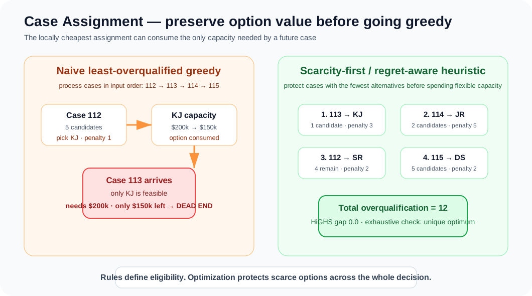
Case 113 is the structural clue. Kevin Jones (KJ) is the only feasible analyst for it, and he has exactly $200,000 of remaining total-case capacity.
That capacity has option value.
Why the obvious greedy rule fails
Suppose we process cases in the input order:
112, 113, 114, 115and assign each case to the currently feasible analyst with the least overqualification.
For case 112, KJ is attractive:
KJ level = 4
case 112 complexity = 3
penalty = 1
So a myopic greedy rule assigns:
112 → KJCase 112 consumes $50,000 of KJ’s $200,000 remaining capacity, leaving $150,000.
Then case 113 arrives. It needs $200,000, and KJ is its only feasible analyst.
The greedy sequence is now infeasible.
Nothing about the first assignment was individually illegal. It was just globally destructive.
A simple heuristic that respects option value
A better constructive heuristic is:
- Recompute feasible candidates for every unassigned case.
- Choose the case with the fewest remaining candidates.
- Break ties using regret: prefer the case where losing its best candidate hurts most.
- Assign the least-overqualified feasible analyst.
- Update residual capacity and repeat.
On this instance the heuristic produces:
| Step | Case | Analyst | Candidate count at selection | Overqualification |
|---|---|---|---|---|
| 1 | 113 | KJ | 1 | 3 |
| 2 | 114 | JR | 2 | 5 |
| 3 | 112 | SR | 4 | 2 |
| 4 | 115 | DS | 5 | 2 |
| Total | 12 |
So the final assignment is:
112 → Sue Rogers (SR)
113 → Kevin Jones (KJ)
114 → Jill Ryan (JR)
115 → Debbie Smith (DS)
Exact validation with HiGHS
I then formulated the assignment as a binary MILP.
Let:
x[c,a] = 1 if case c is assigned to analyst aOnly statically eligible case-analyst pairs need variables.
Every case is assigned exactly once:
sum_a x[c,a] = 1 for every case cFor each analyst, newly assigned case dollars cannot exceed residual capacity:
sum_c amount[c] x[c,a]
    <= max_total[a] - current_amount[a]
The objective is:
min sum_c sum_a
    (level[a] - complexity[c]) x[c,a]
HiGHS returned:
112 → SR
113 → KJ
114 → JR
115 → DS

objective = 12
MIP gap   = 0.0
So the scarcity-first heuristic happened to reach the exact global optimum.
Independent exhaustive check
The instance is small enough to verify without trusting the MILP implementation.
I enumerated all analyst choices, rejected assignments violating eligibility or shared capacity, and found:
40 feasible complete assignments
1 assignment with objective 12
The unique best assignment is the same one returned by HiGHS and the heuristic.
That matches the optimal result reported by the cDMN solution as well.
Executed validation code
from itertools import product
import numpy as np
from scipy.optimize import milp, LinearConstraint, Bounds

analysts = {
    "TS": dict(level=10, current=35000000, max_case=50000000,
               max_total=75000000, areas={"Technology", "Research", "Construction"}),
    "SR": dict(level=5, current=5000000, max_case=1000000,
               max_total=7000000, areas={"Technology", "Research"}),
    "SH": dict(level=8, current=19000000, max_case=20000000,
               max_total=20000000, areas={"Construction", "Research"}),
    "JR": dict(level=9, current=14700000, max_case=1500000,
               max_total=25000000, areas={"Technology", "Research", "Construction"}),
    "DS": dict(level=6, current=8000000, max_case=10000000,
               max_total=10000000, areas={"Research", "Technology"}),
    "DB": dict(level=7, current=6000000, max_case=1000000,
               max_total=7500000, areas={"Technology", "Research"}),
    "KJ": dict(level=4, current=2800000, max_case=3000000,
               max_total=3000000, areas={"Research", "Technology"}),
    "RH": dict(level=2, current=850000, max_case=300000,
               max_total=1000000, areas={"Construction", "Technology"}),
}

level_range = {
    1: (1, 2), 2: (1, 2), 3: (1, 2), 4: (1, 3), 5: (2, 3),
    6: (2, 4), 7: (2, 4), 8: (3, 4), 9: (3, 5), 10: (4, 5),
}

cases = {
    112: dict(amount=50000, complexity=3, type="Technology"),
    113: dict(amount=200000, complexity=1, type="Technology"),
    114: dict(amount=1500000, complexity=4, type="Construction"),
    115: dict(amount=300000, complexity=4, type="Research"),
}


def eligible(a, c):
    A = analysts[a]
    C = cases[c]
    low, high = level_range[A["level"]]

    return (
        C["type"] in A["areas"]
        and C["amount"] <= A["max_case"]
        and low <= C["complexity"] <= high
        and A["current"] + C["amount"] <= A["max_total"]
    )


def penalty(c, a):
    return analysts[a]["level"] - cases[c]["complexity"]


# --- Scarcity-first heuristic ---
remaining = {
    a: analysts[a]["max_total"] - analysts[a]["current"]
    for a in analysts
}

unassigned = set(cases)
heuristic = {}

while unassigned:
    choices = []

    for c in sorted(unassigned):
        candidates = [
            a for a in analysts
            if eligible(a, c) and cases[c]["amount"] <= remaining[a]
        ]

        ranked = sorted((penalty(c, a), a) for a in candidates)
        regret = float("inf") if len(ranked) == 1 else ranked[1][0] - ranked[0][0]

        choices.append((len(ranked), -regret, -cases[c]["amount"], c, ranked))

    _, _, _, c, ranked = min(choices)
    _, a = ranked[0]

    heuristic[c] = a
    remaining[a] -= cases[c]["amount"]
    unassigned.remove(c)

print(heuristic)
# {113: 'KJ', 114: 'JR', 112: 'SR', 115: 'DS'}
print(sum(penalty(c, a) for c, a in heuristic.items()))
# 12


# --- Exact MILP ---
case_ids = list(cases)
analyst_ids = list(analysts)

pairs = [
    (c, a)
    for c in case_ids
    for a in analyst_ids
    if eligible(a, c)
]
idx = {pair: i for i, pair in enumerate(pairs)}
n = len(pairs)

objective = np.array([penalty(c, a) for c, a in pairs], dtype=float)
rows, lower, upper = [], [], []

for c in case_ids:
    row = np.zeros(n)
    for a in analyst_ids:
        if (c, a) in idx:
            row[idx[c, a]] = 1
    rows.append(row)
    lower.append(1)
    upper.append(1)

for a in analyst_ids:
    row = np.zeros(n)
    for c in case_ids:
        if (c, a) in idx:
            row[idx[c, a]] = cases[c]["amount"]

    residual = analysts[a]["max_total"] - analysts[a]["current"]
    rows.append(row)
    lower.append(-np.inf)
    upper.append(residual)

result = milp(
    c=objective,
    integrality=np.ones(n),
    bounds=Bounds(np.zeros(n), np.ones(n)),
    constraints=LinearConstraint(
        np.vstack(rows), np.array(lower), np.array(upper)
    ),
)

exact = {
    c: a
    for (c, a), i in idx.items()
    if result.x[i] > 0.5
}

print(exact)
# {112: 'SR', 113: 'KJ', 114: 'JR', 115: 'DS'}
print(result.fun)      # 12.0
print(result.mip_gap)  # 0.0
The broader lesson
The naive greedy failure is not really about greediness. It is about ignoring the value of preserving future options.
KJ looks attractive for case 112 because the immediate penalty is low. But KJ is interchangeable with several analysts for case 112 and irreplaceable for case 113.
That distinction matters in scheduling, inventory allocation, fulfillment, workforce assignment, production planning, and almost every resource-allocation system I have worked with.
A rule engine can answer:
Who is allowed to take this case?The optimization layer has to answer:
Who should take it, given everything else we may still need to do?Those are different questions.
Solution, heuristic, HiGHS validation, and exhaustive verification by Adam DeJans Jr..
Join the discussion
Sign in with GitHub to leave a comment.