
The July 2026 A Brick Factory challenge asks us to schedule five production orders over an 11-day horizon. Each order must run as one uninterrupted activity, each consumes a fixed number of oven batches per day, and the oven’s available capacity changes over time.
This is a small scheduling problem, but it has the same structure as many real production-planning problems: jobs occupy capacity over multiple periods, capacity is time dependent, and one locally reasonable start time can make the remaining schedule infeasible.
I modeled the problem as a time-indexed mixed-integer linear program (MILP) and solved it with HiGHS.
The solution
HiGHS returned the following feasible schedule:
| Order | Batches/day | Duration | Start | Finish |
|---|---|---|---|---|
| A | 2 | 1 | 9 | 10 |
| B | 1 | 4 | 7 | 11 |
| C | 1 | 4 | 3 | 7 |
| D | 1 | 2 | 0 | 2 |
| E | 2 | 4 | 5 | 9 |
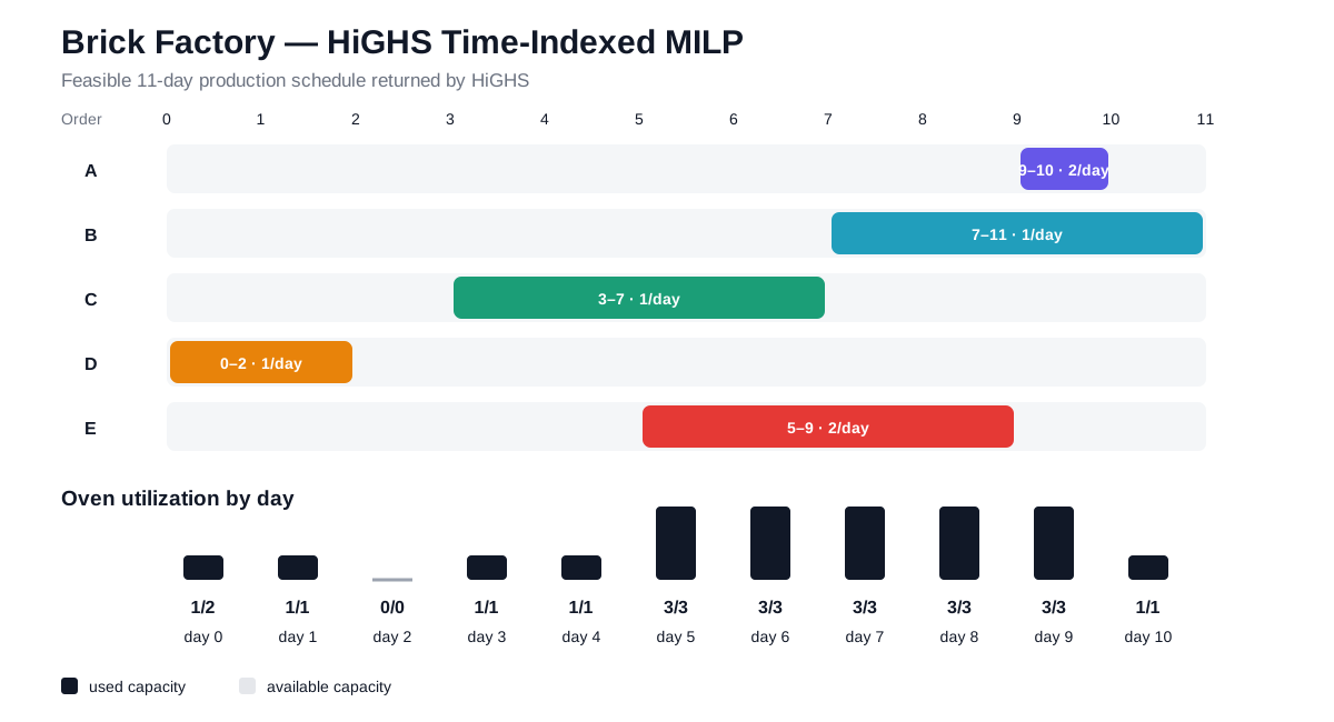
The capacity profile is respected in every period:
| Day | Active orders | Used | Available |
|---|---|---|---|
| 0 | D | 1 | 2 |
| 1 | D | 1 | 1 |
| 2 | — | 0 | 0 |
| 3 | C | 1 | 1 |
| 4 | C | 1 | 1 |
| 5 | C, E | 3 | 3 |
| 6 | C, E | 3 | 3 |
| 7 | B, E | 3 | 3 |
| 8 | B, E | 3 | 3 |
| 9 | A, B | 3 | 3 |
| 10 | B | 1 | 1 |
From day 3 onward the schedule is particularly tight: every period with positive capacity is filled exactly to the oven limit.
The formulation
Define a binary variable x[i,s] that equals 1 when order i starts at day s, and 0 otherwise. Let p[i] be the duration of order i, q[i] its batches per day, and C[t] the oven capacity on day t.
Each order starts exactly once:
sum_s x[i,s] = 1 for every order iAn order that starts at s is active on day t whenever s <= t < s + p[i]. The daily capacity constraints are therefore:
sum_i q[i] * sum_{s: s <= t < s+p[i]} x[i,s] <= C[t]
                                                for every day t
Because the challenge asks only for a feasible schedule, the objective can be zero. The solver simply needs to find a binary assignment satisfying all constraints.
Solving it with HiGHS
I solved the model through SciPy’s milp interface, which uses HiGHS as its mixed-integer optimization backend.
import numpy as np
from scipy.optimize import milp, LinearConstraint, Bounds

H = 11
orders = {
    "A": (2, 1),  # batches/day, duration
    "B": (1, 4),
    "C": (1, 4),
    "D": (1, 2),
    "E": (2, 4),
}
capacity = [2, 1, 0, 1, 1, 3, 3, 3, 3, 3, 1]

# Binary variable for each feasible (order, start-day) pair.
variables = [
    (i, s)
    for i, (_, duration) in orders.items()
    for s in range(H - duration + 1)
]

n = len(variables)
rows, lower, upper = [], [], []

# Every order starts once.
for i in orders:
    row = np.zeros(n)
    for j, (order, _) in enumerate(variables):
        if order == i:
            row[j] = 1
    rows.append(row)
    lower.append(1)
    upper.append(1)

# Daily oven capacity.
for t in range(H):
    row = np.zeros(n)
    for j, (i, s) in enumerate(variables):
        rate, duration = orders[i]
        if s <= t < s + duration:
            row[j] = rate
    rows.append(row)
    lower.append(-np.inf)
    upper.append(capacity[t])

result = milp(
    c=np.zeros(n),
    integrality=np.ones(n),
    bounds=Bounds(np.zeros(n), np.ones(n)),
    constraints=LinearConstraint(
        np.vstack(rows), np.array(lower), np.array(upper)
    ),
    options={"disp": True},
)

for value, (order, start) in zip(result.x, variables):
    if value > 0.5:
        print(order, start)
The formulation contains 26 binary start variables, five start-once constraints, and one capacity condition for each day. The interface simplifies the zero-capacity day before the model reaches the solver, so HiGHS reports 15 rows and 26 columns at the start of presolve. HiGHS then reduced the model to 8 rows and 3 columns, and finally proved feasibility without processing a branch-and-bound node.
The solver report was:
Status            Optimal
Primal bound      0
Dual bound        0
Gap               0%
Solution status   feasible
Nodes             0
For a feasibility model, Optimal means HiGHS found a feasible integer solution and proved the zero objective cannot be improved.
Why time indexing works well here
The formulation is deliberately direct. There are no big-M overlap constraints and no separate continuous start-time variables. Each binary variable already represents a complete scheduling decision: start this order on this day.
The tradeoff is that time-indexed models grow with the planning horizon. For this challenge, that is exactly the right tradeoff. Eleven periods and five orders produce a tiny, transparent model that solves essentially immediately and is easy to verify by inspection.
The same pattern extends naturally to production problems with release dates, due dates, multiple resources, changeovers, or economic objectives such as minimizing tardiness or total production cost.
Solution by Adam DeJans Jr..
Join the discussion
Sign in with GitHub to leave a comment.